ECONOMIC CURVES RELEVANT FOR UPSC

Relevance: Prelims: Economy

►BEVERIDGE CURVE

It is a graphical representation of the relationship between unemployment  (on  the  horizontal axis)  and  job  vacancy rate (on the vertical axis).

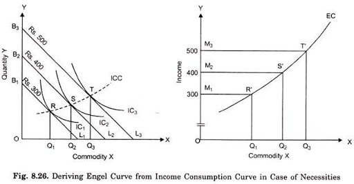
►ENGEL CURVE

It  displays  how  household expenditure  on  a  particular good or service  varies with change in household income.

Eg. As income of a household increases its expenditure of food as a percentage declines. However, its expenditure on status goods increases.

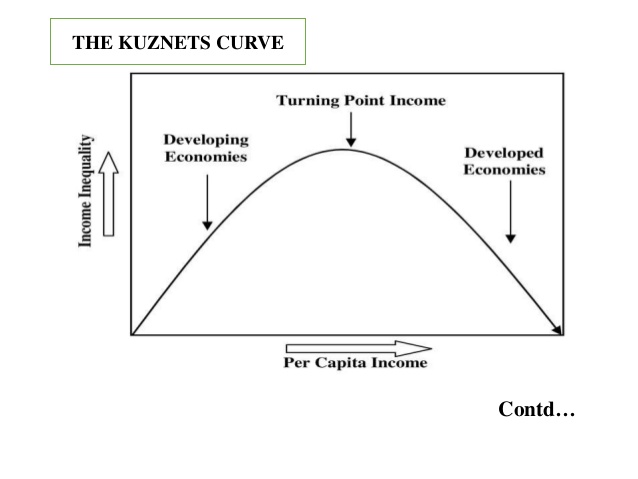
►KUZNETS CURVE

It shows the relationship between economic  growth  and inequality. It is inverted U shaped meaning that as initially economic growth leads to greater inequality, followed later by the reduction of inequality.

►LAFFER CURVE

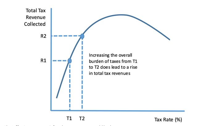
The Laffer Curve is a theory that states lower tax rates boost economic growth. It underpins supply-side economics, Reaganomics, and the Tea Party’s economic policies. Economist Arthur Laffer developed it in 1979.

The Laffer Curve describes how changes in tax rates affect government revenues in two ways. One is immediate, which Laffer describes as “arithmetic.” Every dollar in tax cuts translates directly to one less dollar in government revenue.

The other effect is longer-term, which Laffer describes as the “economic” effect. It works in the opposite direction. Lower tax rates put money into the hands of taxpayers, who then spend it. It creates more business activity to meet consumer demand. For this, companies hire more workers, who then spend their additional income. This boost to economic growth generates a larger tax base. It eventually replaces any revenue lost from the tax cut.

►PHILLIPS CURVE

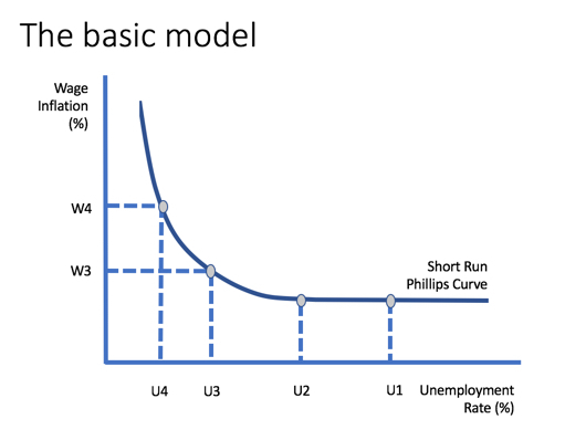
The Phillips curve is an economic concept developed by A. W. Phillips stating that inflation and unemployment have a stable and inverse relationship. The theory claims that with economic growth comes inflation, which in turn should lead to more jobs and less unemployment. However, the original concept has been somewhat disproven empirically due to the occurrence of stagflation in the 1970s, when there were high levels of both inflation and unemployment.

KEY TAKEAWAYS

• The Phillips curve states that inflation and unemployment have an inverse relationship. Higher inflation is associated with lower unemployment and vice versa.
• The Phillips curve was a concept used to guide macroeconomic policy in the 20th century, but was called into question by the stagflation of the 1970’s.
• Understanding the Phillips curve in light of consumer and worker expectations, shows that the relationship between inflation and unemployment may not hold in the long run, or even potentially in the short run.

 

►RAHN CURVE

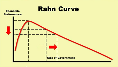
It  displays the  relationship between g overnment spending (on the horizontal) and GDP growth rate (on the vertical) of an economy. It is an inverted U shaped, thus displaying there is a level  of  government  spending  at  whiich  economic  growth theoretically maximises.

 

►ENVIRONMENTAL KUZNET’S CURVE

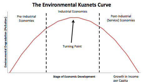
Shows the relationship between economic  progress  and environmental  degradation through time as an economy progresses. As countries develop initiallly, pollution increases, but later, with further development pollution begins to come down. Thus, it is an inverted U-shaped curve.

 

►LORENZ CURVE

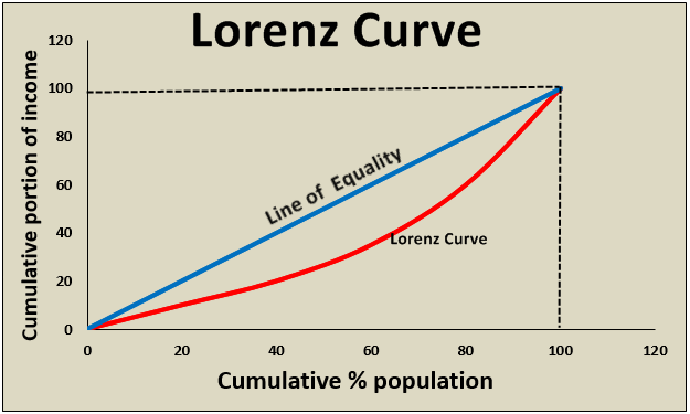
The Lorenz curve is a graphical representation of income inequality or wealth inequality developed by American economist Max Lorenz in 1905. The graph plots percentiles of the population on the horizontal axis according to income or wealth. It plots cumulative income or wealth on the vertical axis, so that an x-value of 45 and a y-value of 14.2 would mean that the bottom 45% of the population controls 14.2% of the total income or wealth.

 

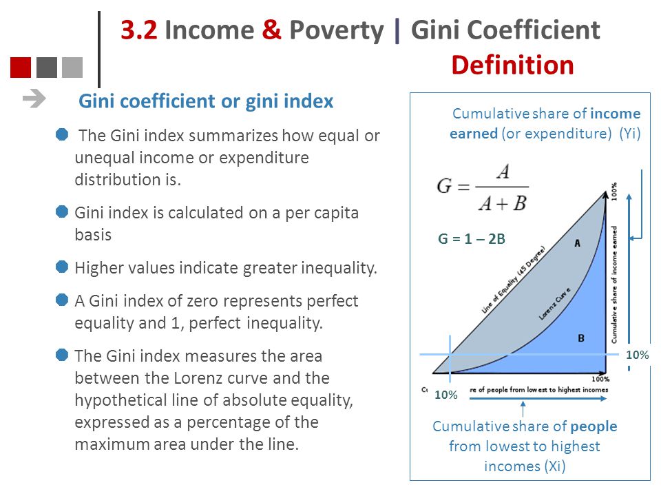
►GINI COEFFICIENT

The Gini index or Gini coefficient is a statistical measure of distribution developed by the Italian statistician Corrado Gini in 1912. It is often used as a gauge of economic inequality, measuring income distribution or, less commonly, wealth distribution among a population. The coefficient ranges from 0 (or 0%) to 1 (or 100%), with 0 representing perfect equality and 1 representing perfect inequality. Values over 1 are theoretically possible due to negative income or wealth.

 

For more such notes, Articles, News & Views Join our Telegram Channel.

https://t.me/triumphias

Click the link below to see the details about the UPSC –Civils courses offered by Triumph IAS. https://triumphias.com/pages-all-courses.php